In this article we will see how to implement a Simple Linear Regression Data Model using Python. We will first explore the mathematical foundations underlying Simple Linear Regression and then proceed with the Python Implementation. We will also evaluate the model using some standard evaluation metrics and then finally use the model to make predictions

Regression Analysis refers to a set of statistical methods used for estimating the relationship between a dependent variable and one or more independent variables. We can then use this relationship to forecast the values of the dependent variable.

Regression can be of two types – Linear and Non Linear. Linear regression refers to the use of a linear model for describing the relationship while Non Linear regression refers to the use of non linear model for describing the same. It is important to note that in case of Linear Regression, the dependent variable should be a continuous variable. However the independent variables can be measured in a continuous or categorical scale.

Linear Regression can be of two types- Simple Linear Regression and Multiple Linear Regression. In Simple Linear Regression we use only independent variable to estimate the value of the dependent variable whereas in Multiple Linear Regression we can use more than one independent variables.

In this article, however we will restrict our discussion to Simple Linear Regression only

1. Mathematical Foundations for Simple Linear Regression

The equation of regression line with 1 dependent variable is represented as:

Y = b_0 + b_1 * X

where b_0 is called the intercept and b_1 is called the Coefficient.

Once we’ve estimated these coefficients, we can use the model to predict responses

2. Understanding the Data

We will use a dataset relating SAT Score and GPA data. We will split the data into training and testing set and use the training set to create a model. We will use the test set to evaluate the model and then finally use the model for predicting the unknown values. SAT Score will be the independent variable and GPA will be the dependent variable. So We would use the model to predict the relative GPA corresponding to SAT Scores.

The data set used in this example can be found here .

3. Python Implementation

The Python Implementation can be broadly divided into following tasks:

• Importing the required Packages and Classes
• Reading the Data
• Splitting the Data into mutually exclusive training set and test set
• Create a model using the Training the data
• Evaluate the model using the test data and several evaluation metrics
• Using the model to predict values

3.1 Importing the required Packages and Classes

We will be using the following packages:

• pandas: It is a software library written for data manipulation and analysis for Python
• numpy: It is a library written for python for providing support for arrays, matrices and a large number of mathematical functions to operate on these arrays
• matplotlib: It is a plotting library for Python
• sklearn: It is a machine learning library for the Python programming language

import pandas as pd;
import numpy as np;
import matplotlib.pyplot as plt;
from sklearn import linear_model;
from sklearn.model_selection import train_test_split;
from sklearn.metrics import r2_score;

3.2 Reading the Data

The dataset used in this example is available in the sat_gpa.csv file (download link already provided) We will use pandas.read_csv method to read the dataset into a Dataframe object

df=pd.read_csv("sat_gpa.csv");

3.3 Splitting the data into training data and test data set

We will randomly split the data so that 90% of the records are used for training the model while the remaining 10% records will be used for testing the model.

train_data, test_data= train_test_split(df,test_size=0.1,random_state=1);
train_data_X = np.asanyarray(train_data[['SAT']]);
train_data_Y = np.asanyarray(train_data[['GPA']]);
test_data_X = np.asanyarray(test_data[['SAT']]);
test_data_Y = np.asanyarray(test_data[['GPA']]);

3.4 Creating the Model

As noted earlier, the coefficient and intercept are the only parameters needed for fitting the line in Simple Linear Regression. We will use the sklearn package to directly estimate these parameters from the training data

lin_reg= linear_model.LinearRegression();
lin_reg.fit(train_data_X, train_data_Y);
reg_coefficient = lin_reg.coef_[0][0];
reg_intercept= lin_reg.intercept_[0];
test_data_Y_hat = lin_reg.predict(test_data_X);
print ("Coefficient ",reg_coefficient);
print ("Intercept ",reg_intercept);

To visualize the fitted line, we plot the line against the training set data as shown below. The training set data points are plotted in blue while the corresponding GPA-value estimates from the model are plotted in red 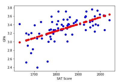The following python code block can be used to plot the above scatter plot

plt.scatter(train_data['SAT'],train_data['GPA'],color='blue');
plt.scatter(train_data['SAT'],train_data['SAT'] * reg_coefficient 
+ reg_intercept,color='red');
plt.xlabel('SAT Score');
plt.ylabel('GPA');
plt.show();

3.5 Model Evaluation

For evaluating the model, we will use the following three metrics

• Mean Absolute Error (MAE): It is the mean of the absolute errors
• Mean Square Error(MSE): Its is the mean of the squared errors and helps to focus on large errors
• Coefficient of Determination (R2 score): It represents how close the data are to the fitted line. Higher the R2 Score, the better is the fit

Following is the python implementation for evaluating the model

MAE=np.mean(np.absolute(test_data_Y_hat - test_data_Y));
MSE=np.mean((test_data_Y_hat - test_data_Y) ** 2);
r2score = r2_score(test_data_Y_hat,test_data_Y);
print("Mean Absolute Error: %0.2f"% MAE );
print("Mean Squared Error (MSE): %0.2f"% MSE );
print ("R2 Score: %0.2f"% r2score);

Following would be the output on executing the above code snippet:

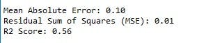
The R2-Score of 0.56 indicates that 56% of the the total variation in the dependent variable (GPA) can be explained by the independent variable (SAT)

In Simple Regression, the value of the dependent variable depends on the value of a single independent variable. But in real life situations, more often than not, we need more than one independent variables to explain the variation in the dependent variable. For example, the price of an apartment may depend on several factors like total size of the apartment, location of the property, the floor on which the apartment is located, the size of the parking lot and so on. None of these variables or factors in isolation can explain the variation in prices in totality, we need to study the effect of all these variables in combination to estimate the variation in prices. In such cases we cannot use Simple Regression. For such cases we have to use another Regression Technique called Multiple Regression.